Testing the GIS library from R, Calculate a SLA concordance
In this post we will use the swish R/PostGIS tools to manipulate spatial data on a remote GIS server (to calculate a SLA concordance) and extract the result to our local client machine. Clink here for the R script.
The great thing about PostGIS is that it is a standard relational database that also understands spatial data. We have developed an R package called swishdbtools to assist connecting to the Database from Kepler.
require(swishdbtools)
ch <- connect2postgres2("gislibrary")
# fill in the details, only required once as will save to your profile
dbGetQuery(ch,
       "select t1.sla_id, t2.sla_code as s2, st_area(t1.geom)
       from abs_sla.nswsla91 t1 join abs_sla.nswsla01 t2
       on t1.sla_id = 1 || substr(cast(t2.sla_code as text), 6,9);
       ")
Pretty cool huh? Spatial functions start with st and the generic name for the spatial data is geom or the_geom.
say we want to create a concordance file to map changes between SLA boundaries
I figured out a complicated SQL syntax to compute the intersecting geometries, then wrapped it up into an R function:
# make a temporary tablename, to avoid clobbering
temp_table <- swish_temptable("gislibrary")
temp_table <- paste("public", temp_table$table, sep = ".")


sql <- postgis_concordance(conn = ch, source_table = "abs_sla.nswsla91",
   source_zones_code = 'sla_id', target_table = "abs_sla.nswsla01",
   target_zones_code = "sla_code",
   into = temp_table, tolerance = 0.01,
   subset_target_table = "cast(sla_code as text) like '105%'",
   eval = F)
cat(sql)
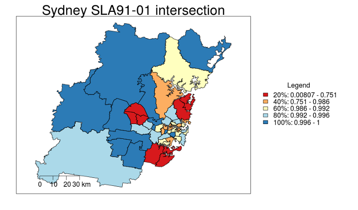
Which gives the map
This shows the SLAs that existed in 2001 that were a smaller segment of their original SLA zone in 1991 (the red areas changed the most).
From the less pretty SQL
I just run the single line version
dbSendQuery(ch, sql)
if I don’t want to look at the ugly code
so now I can use QGIS to visualise this, or if on linux rgdal can access it direct
require(devtools) # windoze users need to install Rtools
install_github("gisviz", "ivanhanigan")
# otherwise download and install from http://ivanhanigan.github.io/gisviz/
require(gisviz)

# get pwd from store, or use pwd <- getPassword()
pwd <- get_passwordTable()
pwd <- pwd[which(pwd$V3 == "gislibrary"), "V5"]

shp <- readOGR2(hostip="130.56.60.77",user="gislibrary",
   db="gislibrary", layer=gsub("public.","",temp_table), p = pwd)
head(arrange(shp@data, prop_olap_src_segment_of_src_orig))
subset(shp@data, source_zone_code == 10750)[,c(1,4,6)]
# source_zone_code target_zone_code prop_olap_src_segment_of_src_orig
# 36            10750        105530751                         0.4791171
# 37            10750        105530752                         0.2455572
# 38            10750        105530753                         0.2726988
# save local copy
writeOGR(shp, "sydneyconc", "sydneyconc", driver="ESRI Shapefile")
# make default map
choropleth(stat="prop_olap_src_segment_of_src_orig", region.map=shp, scalebar = T,
  probs = seq(0, 1, .2), invert.brew.pal= F, maptitle='Sydney SLA91-01 intersection')
and finally just clean up the temp file from the db
dbSendQuery(ch, paste("drop table ",temp_table,sep=""))
